Time Evolution using Renormalizer#
Overview#
In this notebook we will simulate the charge transfer between two molecules using the Marcus model
with transfer integral \(V=-0.1\), dimensionless coupling constant \(g=1\), vibration frequency \(\omega=0.5\).
We will first show how to use Renormalizer to simulation the time evolution at \(\Delta G = 0\). Then, we will show that, by decreasing the reaction Gibbs free energy change \(\Delta G\), the reaction rate will first increase and then decrease, as predicted by the Marcus theory.
Preparation: Setting Up Logger#
[1]:
from renormalizer.utils.log import package_logger as logger
2026-05-20 02:56:51,273[INFO] Use NumPy as backend
2026-05-20 02:56:51,274[INFO] numpy random seed is 9012
2026-05-20 02:56:51,275[INFO] random seed is 1092
2026-05-20 02:56:51,284[INFO] Git Commit Hash: 956ad15b6be989049c1a009a0050334f3d774d43
2026-05-20 02:56:51,285[INFO] use 64 bits
[2]:
logger.debug("logger output")
2026-05-20 02:56:51,325[DEBUG] logger output
[3]:
from renormalizer.utils.log import set_stream_level, INFO
[4]:
# filter logger output
set_stream_level(INFO)
[5]:
logger.debug("This message will not be shown")
[6]:
logger.info("Logger output")
2026-05-20 02:56:51,344[INFO] Logger output
Define the Model and Initial State#
[7]:
from renormalizer import Op, BasisMultiElectron, BasisSHO, Model
import numpy as np
[8]:
v = -0.1
g = 1
omega = 0.5
nbas = 16
[9]:
def get_model(delta_g):
    ham_terms = v * Op(r"a^\dagger a", ["e0", "e1"]) + v * Op(r"a^\dagger a", ["e1", "e0"])
    ham_terms += delta_g * Op(r"a^\dagger a", "e1")
    for i in range(2):
        ham_terms += omega * Op(r"b^\dagger b", f"v{i}")
        ham_terms += g * omega * Op(r"a^\dagger a", f"e{i}") * Op(r"b^\dagger+b", f"v{i}")
    basis = [BasisMultiElectron(["e0", "e1"], [0, 0]), BasisSHO("v0", omega, nbas), BasisSHO("v1", omega, nbas)]
    return Model(basis, ham_terms)
[10]:
# using a relaxed initial state
def get_init_condition():
    basis = BasisSHO(0, omega, nbas)
    state = np.linalg.eigh(basis.op_mat(r"b^\dagger b") + g * basis.op_mat(r"b^\dagger+b"))[1][:, 0]
    return {"v0": state}
init_condition = get_init_condition()
Time Evolution with the Default Configuration#
Next, we run the simulation using the evolve method in the Mps class. At this phase, we keep \(\Delta G = 0\).
[11]:
delta_g = 0
model = get_model(delta_g)
[12]:
from renormalizer import Mps, Mpo
[13]:
# Hamiltonian MPO
mpo = Mpo(model)
# The occupation of e0
n_op = Mpo(model, Op(r"a^\dagger a", "e0"))
[14]:
# initialize the MPS
mps = Mps.hartree_product_state(model, condition=init_condition)
# time evolution step
dt = 0.2
# record the electronic occupation
n_list = []
for i_step in range(50):
    n = mps.expectation(n_op)
    logger.info(f"Step {i_step}. Time {i_step * dt:.2f}. $n$ {n}")
    # perform time evolution. Note that the evolution is not in-place.
    mps = mps.evolve(mpo, dt)
    n_list.append(n)
2026-05-20 02:56:51,396[INFO] Step 0. Time 0.00. $n$ 0.9999999999999998
2026-05-20 02:56:51,410[INFO] Step 1. Time 0.20. $n$ 0.9996030537865594
2026-05-20 02:56:51,421[INFO] Step 2. Time 0.40. $n$ 0.9984313966561619
2026-05-20 02:56:51,435[INFO] Step 3. Time 0.60. $n$ 0.9965532876450579
2026-05-20 02:56:51,451[INFO] Step 4. Time 0.80. $n$ 0.9940731362639054
2026-05-20 02:56:51,466[INFO] Step 5. Time 1.00. $n$ 0.991116186884249
2026-05-20 02:56:51,482[INFO] Step 6. Time 1.20. $n$ 0.9878132450238745
2026-05-20 02:56:51,498[INFO] Step 7. Time 1.40. $n$ 0.9842873078294339
2026-05-20 02:56:51,514[INFO] Step 8. Time 1.60. $n$ 0.9806441927926954
2026-05-20 02:56:51,530[INFO] Step 9. Time 1.80. $n$ 0.976967746624379
2026-05-20 02:56:51,546[INFO] Step 10. Time 2.00. $n$ 0.9733182226560808
2026-05-20 02:56:51,564[INFO] Step 11. Time 2.20. $n$ 0.9697373081106376
2026-05-20 02:56:51,580[INFO] Step 12. Time 2.40. $n$ 0.9662497016753405
2026-05-20 02:56:51,596[INFO] Step 13. Time 2.60. $n$ 0.962867160945706
2026-05-20 02:56:51,612[INFO] Step 14. Time 2.80. $n$ 0.9595919026133962
2026-05-20 02:56:51,629[INFO] Step 15. Time 3.00. $n$ 0.9564197521679629
2026-05-20 02:56:51,645[INFO] Step 16. Time 3.20. $n$ 0.9533423734970324
2026-05-20 02:56:51,661[INFO] Step 17. Time 3.40. $n$ 0.9503492089387038
2026-05-20 02:56:51,677[INFO] Step 18. Time 3.60. $n$ 0.9474287391824951
2026-05-20 02:56:51,695[INFO] Step 19. Time 3.80. $n$ 0.9445692798814911
2026-05-20 02:56:51,712[INFO] Step 20. Time 4.00. $n$ 0.9417594196434944
2026-05-20 02:56:51,728[INFO] Step 21. Time 4.20. $n$ 0.938988314016884
2026-05-20 02:56:51,744[INFO] Step 22. Time 4.40. $n$ 0.9362456942950407
2026-05-20 02:56:51,761[INFO] Step 23. Time 4.60. $n$ 0.9335221984937243
2026-05-20 02:56:51,777[INFO] Step 24. Time 4.80. $n$ 0.9308095732941701
2026-05-20 02:56:51,793[INFO] Step 25. Time 5.00. $n$ 0.9281008849250422
2026-05-20 02:56:51,809[INFO] Step 26. Time 5.20. $n$ 0.9253906107085342
2026-05-20 02:56:51,826[INFO] Step 27. Time 5.40. $n$ 0.9226738471654728
2026-05-20 02:56:51,842[INFO] Step 28. Time 5.60. $n$ 0.9199478805518423
2026-05-20 02:56:51,858[INFO] Step 29. Time 5.80. $n$ 0.9172094618331406
2026-05-20 02:56:51,874[INFO] Step 30. Time 6.00. $n$ 0.9144551950424458
2026-05-20 02:56:51,891[INFO] Step 31. Time 6.20. $n$ 0.9116816732036942
2026-05-20 02:56:51,907[INFO] Step 32. Time 6.40. $n$ 0.9088859026726781
2026-05-20 02:56:51,923[INFO] Step 33. Time 6.60. $n$ 0.9060659656334908
2026-05-20 02:56:51,940[INFO] Step 34. Time 6.80. $n$ 0.90322101218372
2026-05-20 02:56:51,956[INFO] Step 35. Time 7.00. $n$ 0.9003515623906606
2026-05-20 02:56:51,973[INFO] Step 36. Time 7.20. $n$ 0.8974590790192766
2026-05-20 02:56:51,990[INFO] Step 37. Time 7.40. $n$ 0.8945453849965326
2026-05-20 02:56:52,006[INFO] Step 38. Time 7.60. $n$ 0.8916120979060871
2026-05-20 02:56:52,023[INFO] Step 39. Time 7.80. $n$ 0.8886602437062094
2026-05-20 02:56:52,039[INFO] Step 40. Time 8.00. $n$ 0.8856902107426247
2026-05-20 02:56:52,056[INFO] Step 41. Time 8.20. $n$ 0.8827020259679245
2026-05-20 02:56:52,073[INFO] Step 42. Time 8.40. $n$ 0.8796958667524065
2026-05-20 02:56:52,089[INFO] Step 43. Time 8.60. $n$ 0.876672673739856
2026-05-20 02:56:52,105[INFO] Step 44. Time 8.80. $n$ 0.8736347299848458
2026-05-20 02:56:52,122[INFO] Step 45. Time 9.00. $n$ 0.8705861034366976
2026-05-20 02:56:52,139[INFO] Step 46. Time 9.20. $n$ 0.8675328737556515
2026-05-20 02:56:52,155[INFO] Step 47. Time 9.40. $n$ 0.8644830817098144
2026-05-20 02:56:52,172[INFO] Step 48. Time 9.60. $n$ 0.8614463370235248
2026-05-20 02:56:52,188[INFO] Step 49. Time 9.80. $n$ 0.8584330043902285
[15]:
# plotting the occupation
from matplotlib import pyplot as plt
plt.style.use("mm.mplstyle")

plt.plot(np.arange(len(n_list)) * dt, n_list, label="Default")
plt.xlabel("$t$")
plt.ylabel(r"Occupation $\langle a^\dagger_0 a_0 \rangle$")
plt.legend()
plt.show()
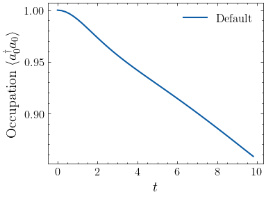
In this example, the time evolution is performed with default time evolution configuration and MPS compression configuration.
Renormalizer by default uses the RK4 “propagation and compression” method for time evolution. The advantage of the method is that it is easy to understand and setup.
Please refer to our recent review for a discussion of the different time evolution schemes.
[16]:
mps.evolve_config.method
[16]:
<EvolveMethod.prop_and_compress: 'P&C'>
Regarding MPS compression/truncation configuration, Renormalizer by default employs a truncation scheme based on the the singular value threshold.
[17]:
mps.compress_config.criteria, mps.compress_config.threshold
[17]:
(<CompressCriteria.threshold: 'threshold'>, 0.001)
Inspection of the dimension of the final mps after time evolution shows that the compression is efficient.
[18]:
mps.bond_dims
[18]:
[1, 2, 4, 1]
Configuring Time Evolution#
In order to configure the time evolution, you should update the evolve_config and compress_config attributes of an MPS instance. These attributes are instances of the EvolveConfig class and the CompressConfig class. Please see the API referece for full options of the configuration classes.
[19]:
from renormalizer.utils.configs import CompressConfig, CompressCriteria
[20]:
# update the compresssion configuration. Adopt a fixed bond dimension of 8
mps.compress_config = CompressConfig(CompressCriteria.fixed, max_bonddim=8)
Next, we perform one more step of the time evolution, and the bond dimension in the middle of the MPS is increased from 4 to 8, according to the updated compression configuration.
[21]:
new_mps = mps.evolve(mpo, dt)
new_mps.bond_dims
[21]:
[1, 2, 8, 1]
Recent studies have shown that methods based on time dependent variantional principle (TDVP) show higher accuracy and efficiency. In our production runs, we usually employ one-site TDVP with projector splitting (TDVP-PS) for time evolution. TDVP-PS allows much larger time evolution step size and reduces memory consumption. However, its setup is a little more complex than propagation and compression, since one-site TDVP generally can not adjust bond dimension during time evolution.
[22]:
from renormalizer.utils.configs import EvolveConfig, EvolveMethod
[23]:
mps.evolve_config = EvolveConfig(EvolveMethod.tdvp_ps)
Next, we perform one more step of the time evolution using TDVP-PS.
Note that the bond dimension in the middle of the MPS does not increase from 4 to 8. This is because one-site TDVP-PS does not alter the bond dimension.
In order to perform one-site TDVP-PS time evolution, it is imperative to increase the bond dimension of the MPS first, and then perform the time evolution.
[24]:
new_mps = mps.evolve(mpo, dt)
new_mps.bond_dims
[24]:
[1, 2, 4, 1]
The expand_bond_dimension function increases the bond dimension to target value specified by the compress_config. In short, the function adds the vectors in the Krylov space \(H^n|\psi\rangle\) to the input wavefunction \(|\psi\rangle\), and then compresses it to the target bond dimension. expand_bond_dimension works with fixed bond dimension compression configuration, instead of singular value truncation threshold.
The include_ex option is specifically designed for systems with quantum number conservation. If the initial wavefunction does not include contributions from a certain symmetry sector, these contributions will not reappear during time evolution due to the projection error in TDVP. Setting include_ex=True will add a small perturbation to the initial state to help recover the missing symmetry sector contributions. In our case, the quantum number conservation is disabled, so we set
include_ex=False.
[25]:
new_mps = mps.expand_bond_dimension(mpo, include_ex=False)
new_mps.bond_dims
[25]:
[1, 2, 8, 1]
Observing Marcus Inverted Region#
Next, we put everything together and perform time evolution with different \(\Delta G\) using TDVP-PS. Since the initial state of time evolution is a Hartree product state, we must expand the bond dimension before performing the time evolution.
[26]:
# time evolution step
dt = 0.5

# initialize the MPS in the Hartree product state
init_mps = Mps.hartree_product_state(model, condition=init_condition)
logger.info(f"Initial MPS bond dimension: {init_mps.bond_dims}")
# setup compression configuration
init_mps.compress_config = CompressConfig(CompressCriteria.fixed, max_bonddim=8)
# setup time evolution configuration
init_mps.evolve_config = EvolveConfig(EvolveMethod.tdvp_ps)


# record the electronic occupation
n_list_list = []

delta_g_list = np.linspace(0, -2, 5)
for delta_g in delta_g_list:
    # reconstruct the Hamiltonian. We can reuse the occupation operator though
    model = get_model(delta_g)
    mpo = Mpo(model)
    # since using TDVP-PS, expand the bond dimension to target value.
    # otherwise the time evolution is limited to the Hartree product state.
    mps = init_mps.expand_bond_dimension(mpo, include_ex=False)
    logger.info(f"MPS bond dimension after expanding: {mps.bond_dims}")
    n_list = []
    for i_step in range(20):
        n = mps.expectation(n_op)
        logger.info(f"Step {i_step}. Time {i_step * dt:.2f}. $n$ {n}")
        # perform time evolution. Note that the evolution is not in-place.
        mps = mps.evolve(mpo, dt)
        n_list.append(n)
    n_list_list.append(n_list)
2026-05-20 02:56:54,662[INFO] Initial MPS bond dimension: [1, 1, 1, 1]
2026-05-20 02:56:54,684[INFO] MPS bond dimension after expanding: [1, 2, 8, 1]
2026-05-20 02:56:54,686[INFO] Step 0. Time 0.00. $n$ 1.0
2026-05-20 02:56:54,712[INFO] Step 1. Time 0.50. $n$ 0.997577678849608
2026-05-20 02:56:54,737[INFO] Step 2. Time 1.00. $n$ 0.9911341778211981
2026-05-20 02:56:54,762[INFO] Step 3. Time 1.50. $n$ 0.9824981838275654
2026-05-20 02:56:54,788[INFO] Step 4. Time 2.00. $n$ 0.9733283418283656
2026-05-20 02:56:54,813[INFO] Step 5. Time 2.50. $n$ 0.9645218516469742
2026-05-20 02:56:54,838[INFO] Step 6. Time 3.00. $n$ 0.9563382368492208
2026-05-20 02:56:54,863[INFO] Step 7. Time 3.50. $n$ 0.9487304333892206
2026-05-20 02:56:54,889[INFO] Step 8. Time 4.00. $n$ 0.9415533981894383
2026-05-20 02:56:54,914[INFO] Step 9. Time 4.50. $n$ 0.9346400325046184
2026-05-20 02:56:54,939[INFO] Step 10. Time 5.00. $n$ 0.9278351842220711
2026-05-20 02:56:54,965[INFO] Step 11. Time 5.50. $n$ 0.9210298996164081
2026-05-20 02:56:54,990[INFO] Step 12. Time 6.00. $n$ 0.9141749831330701
2026-05-20 02:56:55,015[INFO] Step 13. Time 6.50. $n$ 0.9072563582422932
2026-05-20 02:56:55,041[INFO] Step 14. Time 7.00. $n$ 0.900259128610462
2026-05-20 02:56:55,066[INFO] Step 15. Time 7.50. $n$ 0.893152108534242
2026-05-20 02:56:55,092[INFO] Step 16. Time 8.00. $n$ 0.8858943878575136
2026-05-20 02:56:55,118[INFO] Step 17. Time 8.50. $n$ 0.8784553598367519
2026-05-20 02:56:55,142[INFO] Step 18. Time 9.00. $n$ 0.8708472420517182
2026-05-20 02:56:55,167[INFO] Step 19. Time 9.50. $n$ 0.8631616549410941
2026-05-20 02:56:55,211[INFO] MPS bond dimension after expanding: [1, 2, 8, 1]
2026-05-20 02:56:55,212[INFO] Step 0. Time 0.00. $n$ 1.0000000000000002
2026-05-20 02:56:55,237[INFO] Step 1. Time 0.50. $n$ 0.9975401925879036
2026-05-20 02:56:55,262[INFO] Step 2. Time 1.00. $n$ 0.9906013628490239
2026-05-20 02:56:55,287[INFO] Step 3. Time 1.50. $n$ 0.980248885864029
2026-05-20 02:56:55,311[INFO] Step 4. Time 2.00. $n$ 0.9676593608104573
2026-05-20 02:56:55,336[INFO] Step 5. Time 2.50. $n$ 0.9537696503060077
2026-05-20 02:56:55,361[INFO] Step 6. Time 3.00. $n$ 0.9392072948520958
2026-05-20 02:56:55,386[INFO] Step 7. Time 3.50. $n$ 0.92435861042602
2026-05-20 02:56:55,411[INFO] Step 8. Time 4.00. $n$ 0.9094397848359166
2026-05-20 02:56:55,436[INFO] Step 9. Time 4.50. $n$ 0.8945511232283816
2026-05-20 02:56:55,461[INFO] Step 10. Time 5.00. $n$ 0.8797430038665832
2026-05-20 02:56:55,487[INFO] Step 11. Time 5.50. $n$ 0.86507977982476
2026-05-20 02:56:55,511[INFO] Step 12. Time 6.00. $n$ 0.8506519218071078
2026-05-20 02:56:55,537[INFO] Step 13. Time 6.50. $n$ 0.8365374567180586
2026-05-20 02:56:55,561[INFO] Step 14. Time 7.00. $n$ 0.822768823962594
2026-05-20 02:56:55,586[INFO] Step 15. Time 7.50. $n$ 0.8093300617593495
2026-05-20 02:56:55,610[INFO] Step 16. Time 8.00. $n$ 0.7961632960693853
2026-05-20 02:56:55,635[INFO] Step 17. Time 8.50. $n$ 0.7831685752085126
2026-05-20 02:56:55,660[INFO] Step 18. Time 9.00. $n$ 0.7702000677823148
2026-05-20 02:56:55,685[INFO] Step 19. Time 9.50. $n$ 0.7570646850987605
2026-05-20 02:56:55,730[INFO] MPS bond dimension after expanding: [1, 2, 8, 1]
2026-05-20 02:56:55,731[INFO] Step 0. Time 0.00. $n$ 1.0
2026-05-20 02:56:55,756[INFO] Step 1. Time 0.50. $n$ 0.9975277339592458
2026-05-20 02:56:55,781[INFO] Step 2. Time 1.00. $n$ 0.990426183975138
2026-05-20 02:56:55,805[INFO] Step 3. Time 1.50. $n$ 0.979526804706868
2026-05-20 02:56:55,830[INFO] Step 4. Time 2.00. $n$ 0.965917044906082
2026-05-20 02:56:55,854[INFO] Step 5. Time 2.50. $n$ 0.950685008940619
2026-05-20 02:56:55,879[INFO] Step 6. Time 3.00. $n$ 0.9347455146607793
2026-05-20 02:56:55,903[INFO] Step 7. Time 3.50. $n$ 0.9187422726641736
2026-05-20 02:56:55,928[INFO] Step 8. Time 4.00. $n$ 0.9030158921696054
2026-05-20 02:56:55,953[INFO] Step 9. Time 4.50. $n$ 0.8876520609099666
2026-05-20 02:56:55,978[INFO] Step 10. Time 5.00. $n$ 0.8725982798020393
2026-05-20 02:56:56,002[INFO] Step 11. Time 5.50. $n$ 0.8577742342547106
2026-05-20 02:56:56,027[INFO] Step 12. Time 6.00. $n$ 0.8431151893155991
2026-05-20 02:56:56,052[INFO] Step 13. Time 6.50. $n$ 0.8285809886892007
2026-05-20 02:56:56,077[INFO] Step 14. Time 7.00. $n$ 0.8141772509631175
2026-05-20 02:56:56,101[INFO] Step 15. Time 7.50. $n$ 0.7999687732355235
2026-05-20 02:56:56,127[INFO] Step 16. Time 8.00. $n$ 0.7860556760297732
2026-05-20 02:56:56,151[INFO] Step 17. Time 8.50. $n$ 0.7725203376680703
2026-05-20 02:56:56,176[INFO] Step 18. Time 9.00. $n$ 0.7593659426880218
2026-05-20 02:56:56,201[INFO] Step 19. Time 9.50. $n$ 0.7464615604976049
2026-05-20 02:56:56,245[INFO] MPS bond dimension after expanding: [1, 2, 8, 1]
2026-05-20 02:56:56,246[INFO] Step 0. Time 0.00. $n$ 1.0
2026-05-20 02:56:56,271[INFO] Step 1. Time 0.50. $n$ 0.9975406090105959
2026-05-20 02:56:56,296[INFO] Step 2. Time 1.00. $n$ 0.9906249611406748
2026-05-20 02:56:56,320[INFO] Step 3. Time 1.50. $n$ 0.9804700824710465
2026-05-20 02:56:56,345[INFO] Step 4. Time 2.00. $n$ 0.9686190882357235
2026-05-20 02:56:56,369[INFO] Step 5. Time 2.50. $n$ 0.9564506630039297
2026-05-20 02:56:56,394[INFO] Step 6. Time 3.00. $n$ 0.9448244017405041
2026-05-20 02:56:56,419[INFO] Step 7. Time 3.50. $n$ 0.9339798618065536
2026-05-20 02:56:56,444[INFO] Step 8. Time 4.00. $n$ 0.9236970054402215
2026-05-20 02:56:56,468[INFO] Step 9. Time 4.50. $n$ 0.9136118419963752
2026-05-20 02:56:56,493[INFO] Step 10. Time 5.00. $n$ 0.9034945341198822
2026-05-20 02:56:56,518[INFO] Step 11. Time 5.50. $n$ 0.8933290940558765
2026-05-20 02:56:56,542[INFO] Step 12. Time 6.00. $n$ 0.8832123669566802
2026-05-20 02:56:56,567[INFO] Step 13. Time 6.50. $n$ 0.8732206640791118
2026-05-20 02:56:56,592[INFO] Step 14. Time 7.00. $n$ 0.8633414313596104
2026-05-20 02:56:56,616[INFO] Step 15. Time 7.50. $n$ 0.8534881635602461
2026-05-20 02:56:56,641[INFO] Step 16. Time 8.00. $n$ 0.8435889215796821
2026-05-20 02:56:56,665[INFO] Step 17. Time 8.50. $n$ 0.8336922458093314
2026-05-20 02:56:56,690[INFO] Step 18. Time 9.00. $n$ 0.8239993933201377
2026-05-20 02:56:56,715[INFO] Step 19. Time 9.50. $n$ 0.8147658344265765
2026-05-20 02:56:56,759[INFO] MPS bond dimension after expanding: [1, 2, 8, 1]
2026-05-20 02:56:56,760[INFO] Step 0. Time 0.00. $n$ 1.0000000000000002
2026-05-20 02:56:56,785[INFO] Step 1. Time 0.50. $n$ 0.9975784978846653
2026-05-20 02:56:56,809[INFO] Step 2. Time 1.00. $n$ 0.9911783314788783
2026-05-20 02:56:56,834[INFO] Step 3. Time 1.50. $n$ 0.9828793267407638
2026-05-20 02:56:56,858[INFO] Step 4. Time 2.00. $n$ 0.9748047375106139
2026-05-20 02:56:56,883[INFO] Step 5. Time 2.50. $n$ 0.9681008008243933
2026-05-20 02:56:56,907[INFO] Step 6. Time 3.00. $n$ 0.9626946118364346
2026-05-20 02:56:56,932[INFO] Step 7. Time 3.50. $n$ 0.9578334887382827
2026-05-20 02:56:56,957[INFO] Step 8. Time 4.00. $n$ 0.9528636883612412
2026-05-20 02:56:56,981[INFO] Step 9. Time 4.50. $n$ 0.9476402488995223
2026-05-20 02:56:57,006[INFO] Step 10. Time 5.00. $n$ 0.9423714783197245
2026-05-20 02:56:57,031[INFO] Step 11. Time 5.50. $n$ 0.9372226613912149
2026-05-20 02:56:57,056[INFO] Step 12. Time 6.00. $n$ 0.932143487391272
2026-05-20 02:56:57,080[INFO] Step 13. Time 6.50. $n$ 0.9270168710222628
2026-05-20 02:56:57,105[INFO] Step 14. Time 7.00. $n$ 0.9218472771188868
2026-05-20 02:56:57,130[INFO] Step 15. Time 7.50. $n$ 0.9167421622570106
2026-05-20 02:56:57,154[INFO] Step 16. Time 8.00. $n$ 0.9117276598161894
2026-05-20 02:56:57,179[INFO] Step 17. Time 8.50. $n$ 0.9066479717963576
2026-05-20 02:56:57,204[INFO] Step 18. Time 9.00. $n$ 0.9013355144433673
2026-05-20 02:56:57,229[INFO] Step 19. Time 9.50. $n$ 0.8959335401185677
By plotting the figure, we see that when \(\Delta G=-1\), the charge transfer rate is highest.
[27]:
t = np.arange(len(n_list_list[0])) * dt
for i, n_list in enumerate(n_list_list):
    label = r"$\Delta G =" + str(delta_g_list[i]) + "$"
    plt.plot(t, n_list, label=label, linestyle="--")
plt.xlabel("$t$")
plt.ylabel(r"Occupation $\langle a^\dagger_0 a_0 \rangle$")
plt.legend()
[27]:
<matplotlib.legend.Legend at 0x7f7099e59ee0>
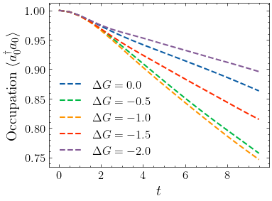
The prediction is consistent with the Marcus theory ,where the Marcus rate is
Here \(\lambda = 2g^2\omega = 1\) is the reorganization energy.
Features of Time Evolution Schemes#
Renormalizer has a lot of different time evolution schemes, the most commonly used ones are 1. Propagation and Compression: EvolveMethod.prop_and_compress 2. Single-site TDVP-PS: EvolveMethod.tdvp_ps 3. Two-site TDVP-PS: EvolveMethod.tdvp_ps2 4. TDVP with varianble mean field (VMF): EvolveMethod.tdvp_vmf
The features of these methods are as follows
Name |
Accuracy |
Computational Cost |
Adaptive Step-Size |
Adaptive Bond Dimension |
Projection Error |
|---|---|---|---|---|---|
|
Low |
High |
partial |
Yes |
No |
|
High |
Low |
No |
No |
Yes |
|
High |
High |
No |
Yes |
Partial |
|
High |
High |
Yes |
No |
Yes |
“Adaptive Step-Size” refers to the ability to dynamically adjust the time-evolution step size based on a predefined error threshold. In practice, this means the method automatically takes smaller steps when the wavefunction changes abruptly and larger steps when it evolves smoothly. For example, tdvp_vmf performs multiple small steps within a single call to the evolve method. This capability removes the need for users to manually check step-size convergence in TD-DMRG by testing multiple
step sizes.
“Adaptive Bond Dimension” refers to the ability to dynamically adjust the bond dimension during time evolution. Typically, the initial state is a Hartree product state. For tdvp_ps and tdvp_vmf, the expand_bond_dimension method should be called before starting the time evolution. Otherwise, the simulation will proceed with a bond dimension of 1 rather than the value specified in the optimization settings.
“Projection Error” is the error introduced when projecting the time derivative onto the MPS manifold.
Empirically, we recommend tdvp_ps for production level calculations.
[ ]: